“Yaar matlab kyon?!”
… is a sentiment expressed by every student who has slogged through an introductory course on statistics. You plow your way through mean, median and mode for the five thousandth time, you nod your head throughout the tedium that is the discussion on the measure of central dispersion, and you get the fact that the sample and population are different things. So far so good.
But then the professor plonks down the formula for standard deviation, and for the first time in your life (but not the last! Oh dear me no, anything but last) you see n-1 in the denominator.
And if it isn’t the class immediately after lunch, and if you are attending instead of bunking, there is a non-zero chance that you will, at worst, idly wonder about the n-1. At best, you might raise a timid hand and ask why it is n-1 rather than simply n.
Historically, students in colleges are likely to be met with one of three explanations.
One:
“That’s the formula”. This is why you’re better off bunking rather than attending these kind of classes.
Two:
“You do divide by n, but in the case of the population standard deviation. This is the formula for the sample standard deviation”. You hear this explanation, and warily look around the class for support, for the battle clearly isn’t over. You know that you should be asking a follow-up question. But that much needed support is not forthcoming. Everybody else is studiously noting something of critical importance in their notebooks. “OK, thank you, Sir”, you mumble, and decide that you’re better off bunking more often.
Three:
“Because you lose one degree of freedom, no?”, the professor says, in a manner which clearly suggests that this ought to be bleedin’ obvious, and can we please get on with it. “Ah, yes, of course”, you respond, not even bothering to check for support. And you decide the obvious, but we knew where this was going already, didn’t we?
So what is this “degrees of freedom” business?
Here’s an explanation in three parts.
First, simple thought experiment. Pick any three numbers. Done? Cool.
Now, pick any three numbers such that they add up to ten. Done? Cool.
In the second case, how many numbers were you free to pick? If you say “three”, imagine me standing in front of you, raised eyebrow and all. “Really, three?” I would have said if was actually there. “Let’s say the first number is 5, and the second number is 3. Are you free to pick the third number?”
And you aren’t, of course. If the first number is 5 and the second number is 3 and the three numbers you pick must add up to 10, then the third number has to be…
2. Of course.
But here’s the point. The imposition of a constraint in this little exercise means you’ve lost a degree of freedom.
Here are some examples from your day to day life:
“Leave any time you like, but make sure you get home by tem pm”. Not much of a “leave any time you like” then, is it? Congratulations, you’ve lost a degree of freedom.
“You can buy anything you want, so long as it is less than a thousand rupees”.
“You can do what you like for the rest of the evening, but only after you finish all your homework”.
The imposition of a constraint implies the loss of a degree of freedom.
Got that? That was the first part of the explanation. Now on to the second part.
So ok, you now know what a degree of freedom is. It is the answer to the question “In a n-step process, how many steps am I free to choose?”. Note that this is not a technically correct explanation, and those howls of outrage you hear are statistics professors reading this and going “Dude, wtf!”. But ignore the background noise, and let’s move on.
But why does the sample standard deviation lose a degree of freedom? Why doesn’t the population standard deviation lose a degree of freedom?
Today’s a good day for thought experiments, so let’s indulge in one more. Imagine that you stay in Bangalore, and that you have to take a rickshaw and then the metro to reach your workplace. It takes you about twenty minutes to find a rickshaw, sit in it, swear at Bangalore’s traffic, and reach the metro. If you’re lucky it takes only fifteen minutes, and if you’re unlucky, it takes thirty. But usually, twenty.
It takes you about forty minutes to get into the metro, get off from the metro and walk to your office. If you’re lucky, thirty five minutes, and if you’re unlucky, forty five minutes. But usually, forty.
If reaching on time is of the utmost importance, and you have to reach by ten am, when should you leave home?
Nine am would be risky, right? You’ve left yourself with zero degrees of freedom in terms of potential downsides. If either the rickshaw ride or the metro ride end up going a little bit over the usual, you’ll have a Very Angry Boss waiting for you.
But late night parties are late night parties, snooze buttons are snooze buttons, and here you are at nine am, hoping against hope that things work out fine. But alas, the rickshaw ride ends up taking twenty five minutes.
Now that the rickshaw ride has ended up taking twenty five, you have only thirty five minutes for the metro part of your journey. You used up some degrees of freedom on the first leg of the journey, and you have none left for the second.
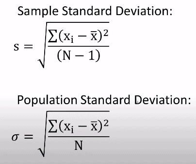
Go look at that formula shown up above. Well, both formulas. What does x-bar stand for? Average, of course. Ah, but of the sample or the population? Any student who has ratta maaroed the formulas will tell you that this is the sample average. The population wala thingummy is called “mu”.
Ab, but now hang on. You’re saying that you want to understand what the population standard deviation looks like, and you’re going to form an idea for what it looks like by calculating the sample standard deviation. But the sample standard deviation itself depends upon your idea of what the population mean looks like. And where did you get an idea for what the population mean looks like? From the sample mean, of course!
But what if the sample mean is a little off? That is, what if the sample mean isn’t exactly like the population mean? Well, let’s keep one data point with us. If it turns out to be off, we’ll have that last data point be such that when you add it to the calculation of the sample mean, we will guarantee that the answer is eggjhactlee equal to the population mean. Hah!
Well ok, but that does then mean that you have… drumroll please… lost one degree of freedom.
In much the same way that taking more time on the rickshaw leg means you can’t take time on the metro leg…
Keeping one datapoint in hand when it comes to the mean implies that you lose that one degree of freedom when it comes to the sample standard deviation.
And that is why you have n-1 degrees of freedom.
I said three parts, remember? So what’s the third bit? If you think you’ve understood what I’ve said, go find someone to explain it to, and check if they get it. Only then, as <insert famous meme of your choice here> says, have you really understood it.
